Machine Learning: California Housing Price

Machine Learning

I analyzed the Callifornia Housing dataset using Python and Machine Learning models to estimate the price of houses. The dataset was obtained from the 1997 book "Sparse Spatial Autoregressions," Statistics and Probability Letters by Pace, R. Kelley, and Ronald Barry. The data itself came from the 1990 Census data. The information was collected on variables at the block group level.

I first started by imported all packages that will be needed , import the data from the CSV file, and then get some summary of the data.

import pandas as pd
import numpy as np

# Data Visualization
import matplotlib.pyplot as plt
plt.style.use('seaborn')
import matplotlib.image as mpimg # To import maps and set them as background

import seaborn as sns

import plotly.express as px

# Machine Learning
from sklearn.linear_model import LinearRegression
from sklearn.linear_model import LogisticRegression
from sklearn.ensemble import RandomForestRegressor
from sklearn import metrics
from sklearn.metrics import mean_squared_error

import scipy.stats as stats

blocks = pd.read_csv('housing.csv')
blocks.head()

blocks.info()

This dataset is almost perfectly cleaned with the except of 207 missing values in total_bedrooms.

blocks.columns

Index(['longitude', 'latitude', 'housing_median_age', 'total_rooms',
'total_bedrooms', 'population', 'households', 'median_income',
'median_house_value', 'ocean_proximity'],
dtype='object')

Looking at blocks with missing values in bedrooms.

blocks_na = blocks[blocks.total_bedrooms.isna()]
blocks_na.head()

blocks_na.ocean_proximity.value_counts()

<1H OCEAN 102
INLAND 55
NEAR OCEAN 30
NEAR BAY 20
Name: ocean_proximity, dtype: int64

blocks[blocks.duplicated()]

There are no duplicates in the dataset.

blocks.describe()

blocks.describe(include = 'O') #To describe categorical columns

blocks.ocean_proximity.value_counts()

<1H OCEAN 9136
INLAND 6551
NEAR OCEAN 2658
NEAR BAY 2290
ISLAND 5
Name: ocean_proximity, dtype: int64

blocks.total_rooms.value_counts().head()

1527.00      18
1613.00      17
1582.00      17
2127.00      16
1703.00      15
Name: total_rooms, dtype: int64

blocks.total_bedrooms.value_counts().head()

280.00 55
331.00      51
345.00      50
393.00      49
343.00      49
Name: total_bedrooms, dtype: int64

Exploratory Visualization

sns.pairplot(blocks)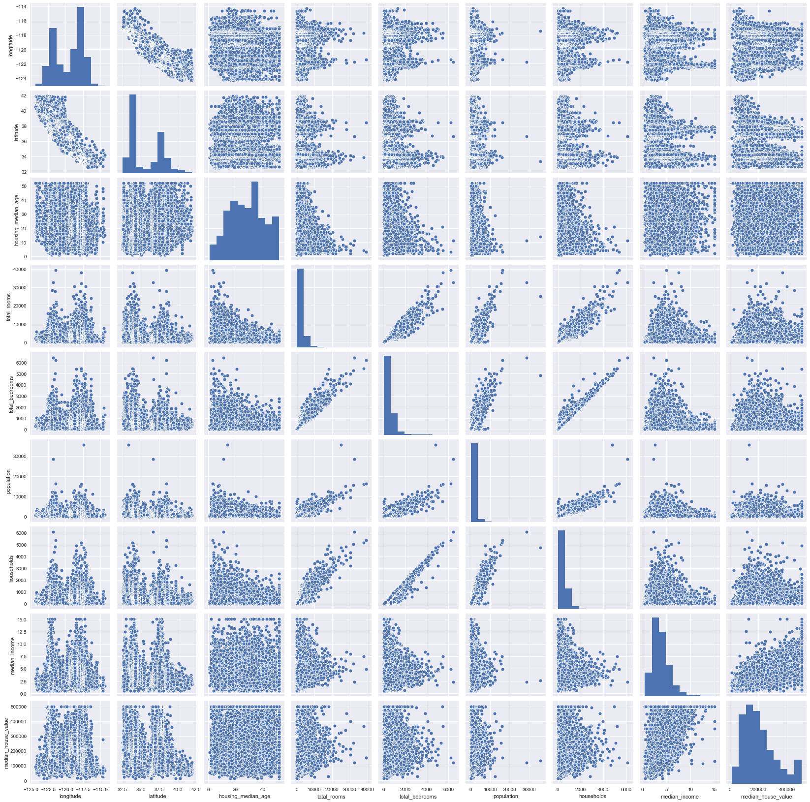

# Creating an histogram for each numerical feature
blocks.hist(bins = 50, figsize = (20,15))
plt.title("Histogram of all numerical features")
plt.figtext(0.5, 0.01, "Data analyzed by Ashek Ag Mohamed", wrap=True, horizontalalignment='center', fontsize=12)
plt.show()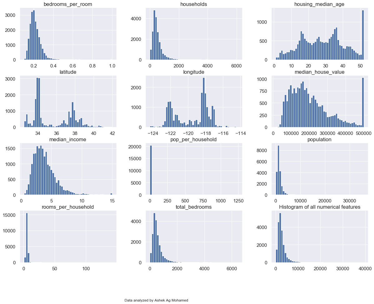

Data Cleaning and Creation of Additional Features

I will drop the missing values here. However, I better approach later on will be to replace them with the median values in a specific category they belong into instead of removing 10% of the dataset.

blocks.dropna(inplace = True)
blocks['rooms_per_household'] = blocks.total_rooms.div(blocks.households)
blocks.head()

# Extreme rooms per household values
blocks.rooms_per_household.nlargest(10)

1914 141.909091
1979 132.533333
12447 62.422222
1913 61.812500
11862 59.875000
1912 56.269231
9676 52.848214
11707 52.690476
2395 50.837838
1240 47.515152
Name: rooms_per_household, dtype: float64

# Extreme rooms per household values
blocks.rooms_per_household.nsmallest(10)

5916 0.846154
8219 0.888889
3126 1.000000
14818 1.130435
17820 1.130435
4552 1.260870
4550 1.378486
4587 1.411290
4602 1.465753
12484 1.550409
Name: rooms_per_household, dtype: float64

blocks['pop_per_household'] = blocks.population.div(blocks.households)
blocks['bedrooms_per_room'] = blocks.total_bedrooms.div(blocks.total_rooms)

Exploratory Data Analysis

blocks.median_house_value.hist(bins=80, figsize = (15,8))
plt.show()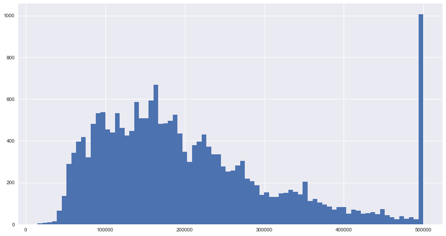

blocks.corr()
blocks.corr().to_csv("block_corr.csv")

	longitude	latitude	housing_median_age	total_rooms	total_bedrooms	population	households	median_income	median_house_value	rooms_per_household
longitude	1	-0.92466	-0.1082	0.044568	0.069608	0.099773	0.05531	-0.01518	-0.04597	-0.02754
latitude	-0.92466	1	0.011173	-0.0361	-0.06698	-0.10878	-0.07104	-0.07981	-0.14416	0.106389
housing_median_age	-0.1082	0.011173	1	-0.36126	-0.32045	-0.29624	-0.30292	-0.11903	0.105623	-0.15328
total_rooms	0.044568	-0.0361	-0.36126	1	0.93038	0.857126	0.918484	0.19805	0.134153	0.133798
total_bedrooms	0.069608	-0.06698	-0.32045	0.93038	1	0.877747	0.979728	-0.00772	0.049686	0.001538
population	0.099773	-0.10878	-0.29624	0.857126	0.877747	1	0.907222	0.004834	-0.02465	-0.07221
households	0.05531	-0.07104	-0.30292	0.918484	0.979728	0.907222	1	0.013033	0.065843	-0.0806
median_income	-0.01518	-0.07981	-0.11903	0.19805	-0.00772	0.004834	0.013033	1	0.688075	0.326895
median_house_value	-0.04597	-0.14416	0.105623	0.134153	0.049686	-0.02465	0.065843	0.688075	1	0.151948
rooms_per_household	-0.02754	0.106389	-0.15328	0.133798	0.001538	-0.07221	-0.0806	0.326895	0.151948	1

blocks.corr().median_house_value.sort_values(ascending = False)

median_house_value 1.000000
median_income 0.688355
rooms_per_household 0.151344
total_rooms 0.133294
housing_median_age 0.106432
households 0.064894
total_bedrooms 0.049686
pop_per_household -0.023639
population -0.025300
longitude -0.045398
latitude -0.144638
bedrooms_per_room -0.255880
Name: median_house_value, dtype: float64

blocks.median_income.hist(bins=80, figsize = (15,8))
plt.show()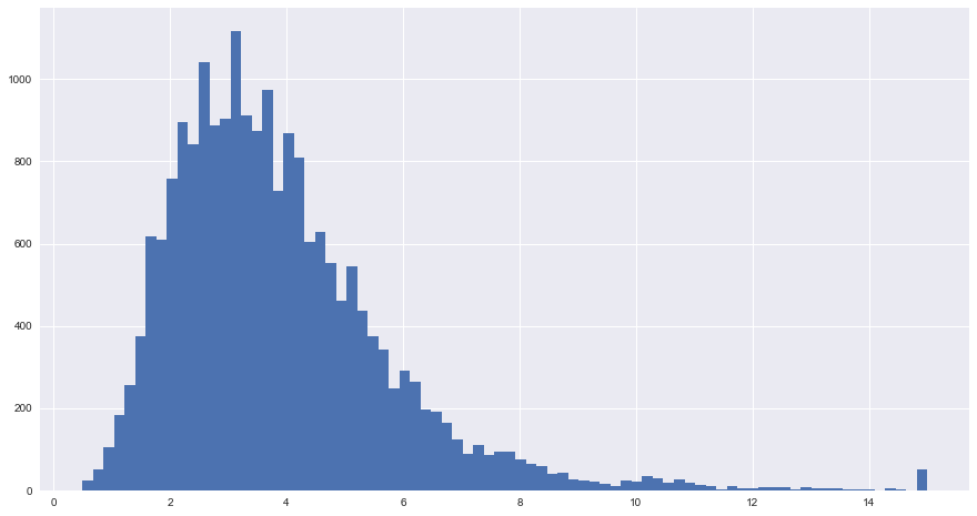

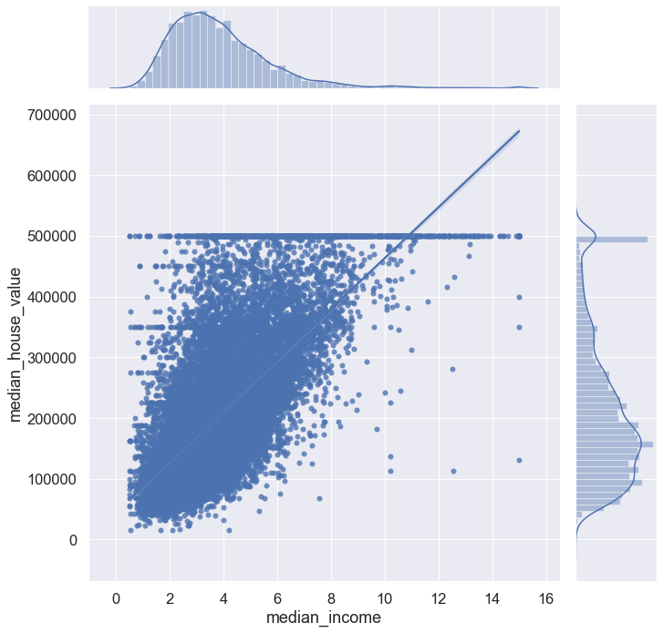
sns.set(font_scale = 1.5)
sns.jointplot(data = blocks, x = 'median_income', y = 'median_house_value', kind = 'kde', height = 10) #kernel density estim.
plt.show()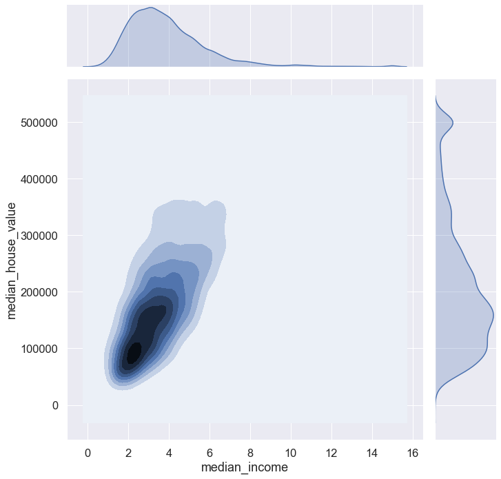

blocks.plot(kind = 'scatter', x = 'longitude', y = 'latitude', 
          s = blocks.population/100, label = 'Population', figsize = (15,10),
          c = 'median_house_value', cmap = 'coolwarm',
          colorbar = True, alpha = 0.4, fontsize = 15, sharex = False
         )
plt.ylabel('Latitude', fontsize = 14)
plt.xlabel('Longitude', fontsize = 14)
plt.legend(fontsize = 16)
plt.show()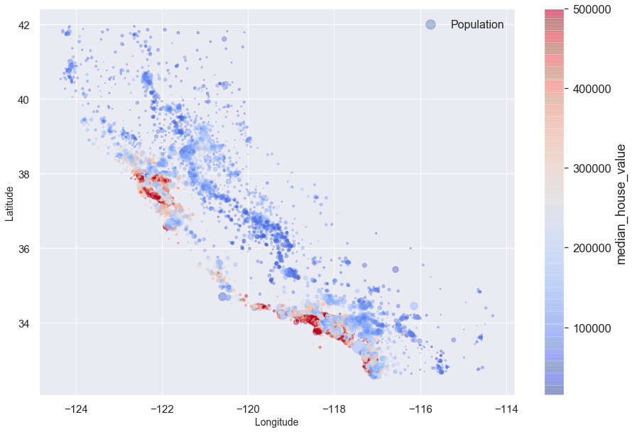

Importing the California Map

california_img = mpimg.imread('california.png') # Image stored as a numpy array.

plt.figure(figsize = (15,10))
plt.imshow(california_img, extent = [-124.55, -113.80, 32.45, 42.05]) # Including coordinates
plt.show()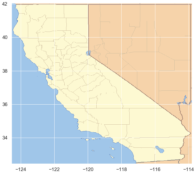

Combining the Map with previous plots

blocks.plot(kind = 'scatter', x = 'longitude', y = 'latitude', 
          s = blocks.population/100, label = 'Population', figsize = (25,15),
          c = 'median_house_value', cmap = 'coolwarm',
          colorbar = True, alpha = 0.4, fontsize = 15, sharex = False
         )

plt.imshow(california_img, extent = [-124.55, -113.80, 32.45, 42.05], alpha = 0.5, 
          cmap = plt.get_cmap('jet'))

plt.ylabel('Latitude', fontsize = 14)
plt.xlabel('Longitude', fontsize = 14)
plt.legend(fontsize = 16)
plt.show()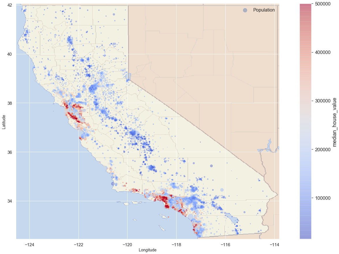

Looking at houses near ocean

prox = blocks.ocean_proximity.unique()
prox

array(['NEAR BAY', '<1H OCEAN', 'INLAND', 'NEAR OCEAN', 'ISLAND'],
dtype=object)

blocks_loc = blocks[blocks.ocean_proximity == prox[3]].copy() # Slices for Near Ocean

blocks_loc.plot(kind = 'scatter', x = 'longitude', y = 'latitude', 
          s = blocks_loc.population/100, label = 'Population', figsize = (25,15),
          c = 'median_house_value', cmap = 'coolwarm',
          colorbar = True, alpha = 0.4, fontsize = 20, sharex = False
         )

plt.imshow(california_img, extent = [-124.55, -113.80, 32.45, 42.05], alpha = 0.5, 
          cmap = plt.get_cmap('jet'))

plt.ylabel('Latitude', fontsize = 14)
plt.xlabel('Longitude', fontsize = 14)
plt.legend(fontsize = 16)
plt.show()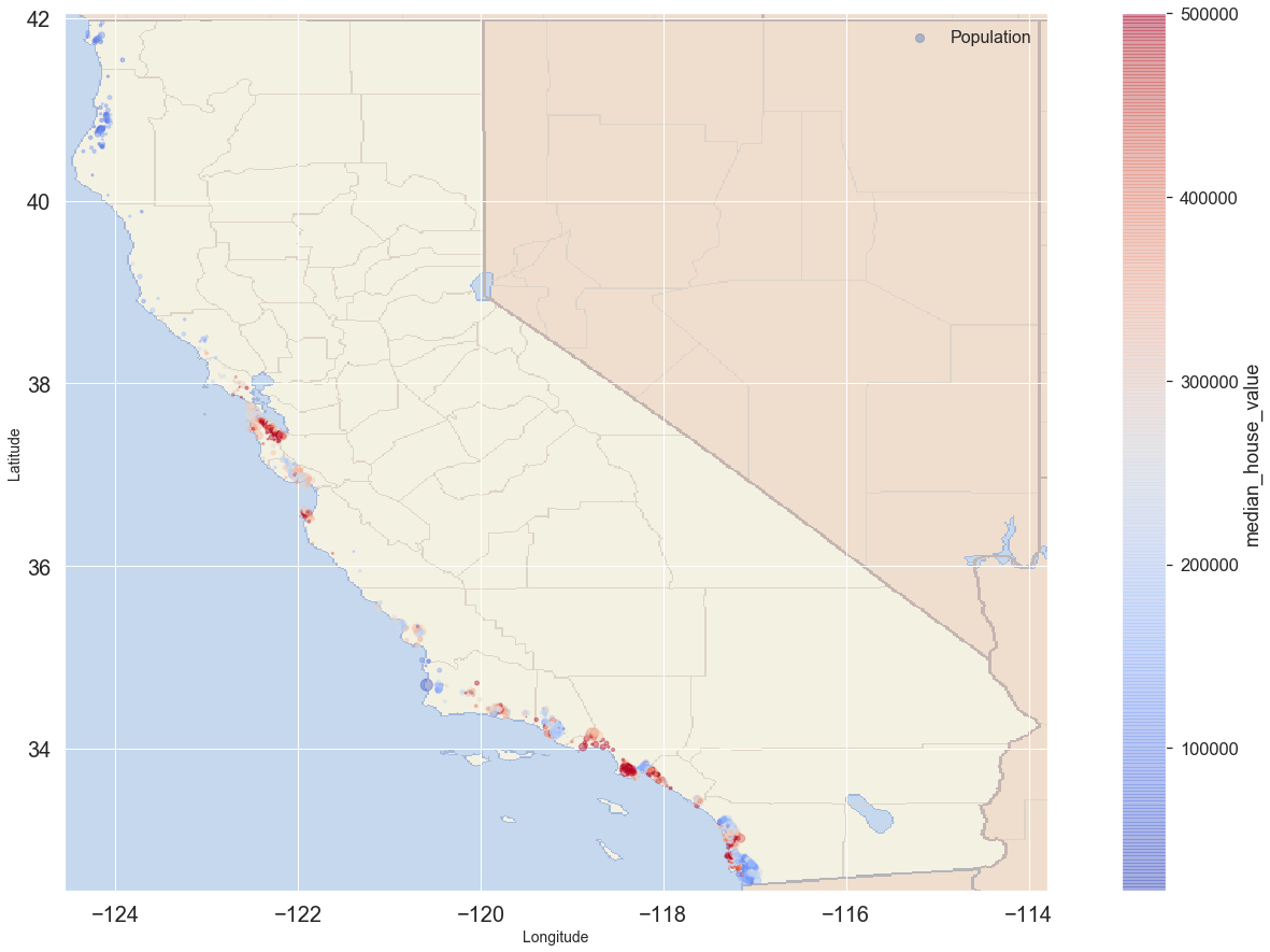

Advanced Exploratory Data Analysis

blocks.median_income.hist(bins=50, figsize = (15,10))
plt.title('Median Income')
plt.show()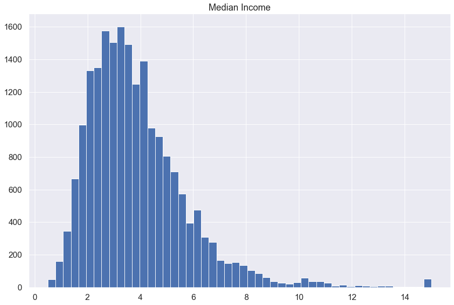

blocks['income_cat'] = pd.qcut(blocks.median_income, q = [0, 0.25, 0.5, 0.75, 0.95, 1], 
                          labels = ['Low', "Below_Average", 'Above_Average', 'High', 'Very_High']) # Categorising income between 5 groups depending on which percentile they fall into.

blocks.income_cat.value_counts(normalize = True)

Above_Average 0.250037
Low 0.250037
Below_Average 0.249988
High 0.199922
Very_High 0.050017
Name: income_cat, dtype: float64

plt.figure(figsize = (12,8))
sns.set(font_scale = 1.5, palette = 'viridis')
sns.countplot(data = blocks, x = 'income_cat', hue = 'ocean_proximity')
plt.legend(loc = 1, fontsize = 14)
plt.show()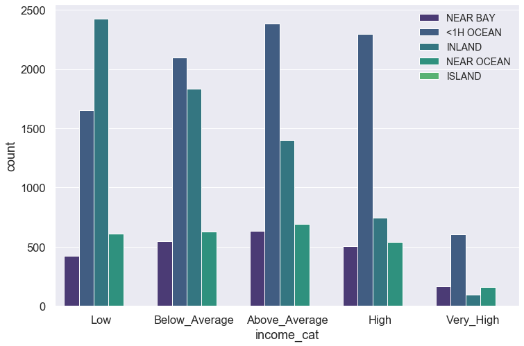

plt.figure(figsize = (13,7))
sns.countplot(x = 'ocean_proximity', hue = 'income_cat', data = blocks, palette = 'viridis')
plt.xlabel('Purpose', fontsize = 15)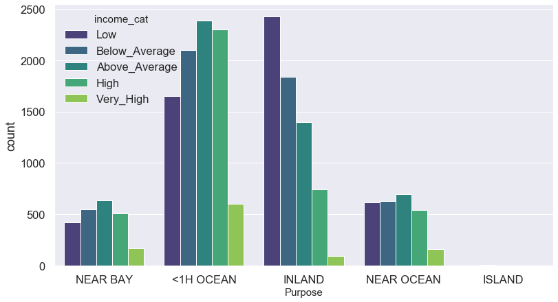

plt.figure(figsize = (12,8))
sns.set(font_scale = 1.5)
sns.barplot(data = blocks, x = 'income_cat', y = 'median_house_value', dodge = True)

plt.show()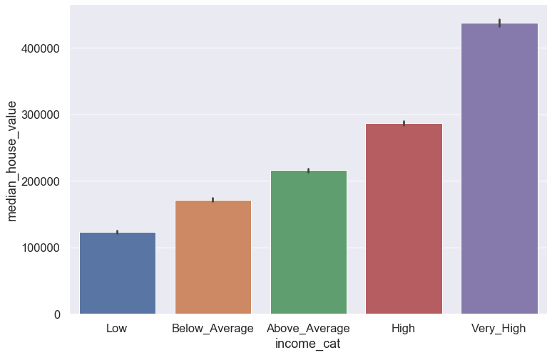

This makes sense in the fact that the median house value increases as the residents' income increases as well.

plt.figure(figsize = (12,8))
sns.set(font_scale = 1.5)
sns.barplot(data = blocks, x = 'ocean_proximity', y = 'median_house_value', dodge = True)

plt.show()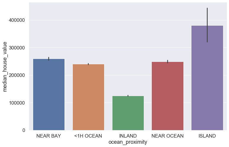

matrix = blocks.groupby(['income_cat', 'ocean_proximity']).median_house_value.mean().unstack().drop(columns = ['ISLAND'])

matrix.astype('int')

plt.figure(figsize = (12,8))
sns.set(font_scale = 1.4)
sns.heatmap(matrix.astype('int'), cmap = 'Reds', annot = True, fmt = 'd', vmin = 90000, vmax = 470000)
plt.show()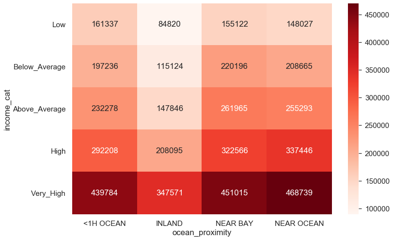

Feature Engineering

Some feature engineering are needed before being able to forecast a machine learning model.

label = blocks.median_house_value.copy() # What to forecast through the model

features = blocks.drop(columns = ['median_house_value']) # Everything else

features.select_dtypes('float')

Numerical features with different scales can negatively impact our machine learning model. Therefore, it is best to standardize them using the z scores.

feat1 = features.select_dtypes('float').apply(lambda x: stats.zscore(x))

pd.options.display.float_format = '{:.2f}'.format # Viewing only two decimal points.

feat1.agg(['mean', 'std'])

The data is standardized because all features have a mean of 0 and a standard deviation of 1.

Some machine learning models cannot handle categorical dataset, so we need to transform them into numerical values.

features.ocean_proximity.value_counts()

<1H OCEAN 9034
INLAND 6496
NEAR OCEAN 2628
NEAR BAY 2270
ISLAND 5
Name: ocean_proximity, dtype: int64

# We use a one hot and coding - using binary values 1 and 0 - to transform categorical features into numerical data types
dummies = pd.get_dummies(features.ocean_proximity)
dummies.head()

# Concatenating our various data
features = pd.concat([feat1, dummies, blocks.income_cat], axis = 1)

Dummiers are redundant because we can determine the value of the last column by looking at the values of the previous one. This multi-colinearity pose a problem to certain machine learning algorythms like the Linear Model and will require deleting one of the columns. The Random Forest model we will use here will not be impacted by this multi-colinearity.

Splitting the Data into Training and Test Set

test_size = 0.2

# Randomly splitting our dataset
X_test = features.sample(frac = test_size, random_state = 123) # fraction = 20% - test_size

X_test.income_cat.value_counts(normalize = True)

Above_Average 0.25
Below_Average 0.25
Low 0.25
High 0.20
Very_High 0.05
Name: income_cat, dtype: float64

features.income_cat.value_counts(normalize = True)

Above_Average 0.25
Low 0.25
Below_Average 0.25
High 0.20
Very_High 0.05
Name: income_cat, dtype: float64

X_test is representative of the dataset, at least when considering the income_cat feature.

X_test.index

Int64Index([14354, 12908, 19545, 12188, 14786, 9941, 3179, 4650, 15550, 17190,
...
3992, 10261, 10862, 10863, 13864, 10262, 3614, 19296, 5826, 15383],
dtype='int64', length=4087)

X_train = features.loc[~features.index.isin(X_test.index)].copy()

X_train = X_train.sample(frac = 1, random_state = 123) # Working with a shuffled data frame

# Don't need the income_cat column for our model
X_train.drop(columns = ['income_cat'], inplace = True)
X_test.drop(columns = ['income_cat'], inplace = True)

y_train = label.loc[X_train.index]
y_test = label.loc[X_test.index]

Training the ML Model (Random Forest Regressor)

forest_reg = RandomForestRegressor(random_state = 42, n_estimators = 500,
                                  max_features = 'sqrt', max_depth = 75, min_samples_split = 2)

forest_reg.fit(X_train, y_train)

RandomForestRegressor(bootstrap=True, ccp_alpha=0.0, criterion='mse',
max_depth=75, max_features='sqrt', max_leaf_nodes=None,
max_samples=None, min_impurity_decrease=0.0,
min_impurity_split=None, min_samples_leaf=1,
min_samples_split=2, min_weight_fraction_leaf=0.0,
n_estimators=500, n_jobs=None, oob_score=False,
random_state=42, verbose=0, warm_start=False)

forest_reg.score(X_train, y_train)

0.9758470860678036

This score is very high and may indicate overfitting.

pred = forest_reg.predict(X_train)
pred

array([238374.608, 246813.8 , 74191.4 , ..., 184930.402, 117595.4 , 187186.008])

forest_mse = mean_squared_error(y_train, pred)
forest_rmse = np.sqrt(forest_mse)
forest_rmse

18023.671210966968

We can conclude that our model fit our training dataset pretty well.

Testing the model with the Test Set

forest_reg.score(X_test, y_test)

0.825152593253362

pred2 = forest_reg.predict(X_test)
pred2

array([224965.808, 129246.8 , 67903. , ..., 222406.402, 322985.02 , 268692.8 ])

forest_mse2 = mean_squared_error(y_test, pred2)
forest_rmse2 = np.sqrt(forest_mse2)
forest_rmse2

47348.34022326726

comp = pd.DataFrame(data = {'True_V':y_test, 'Pred':pred2})
comp

ae = comp.True_V.sub(comp.Pred).abs()
ae

14354 123165.81
12908 83753.20
19545 9103.00
12188 75950.02
14786 13871.60
...
10262 24362.20
3614 7963.20
19296 6506.40
5826 3114.98
15383 22807.20
Length: 4087, dtype: float64

mae = ae.mean()
mae

31722.632696354325

Feature Importance

forest_reg.feature_importances_

array([8.43251997e-02, 7.63824246e-02, 4.20571593e-02, 2.28712182e-02,
2.01285036e-02, 2.28577613e-02, 1.96337714e-02, 2.80813190e-01,
6.50088158e-02, 9.89248218e-02, 9.71199460e-02, 1.91328297e-02,
1.36700488e-01, 2.65441330e-04, 5.35959721e-03, 8.41883258e-03])

feature_imp = pd.Series(data = forest_reg.feature_importances_, index = X_train.columns).sort_values(ascending = False)

feature_imp

median_income 0.28
INLAND 0.14
pop_per_household 0.10
bedrooms_per_room 0.10
longitude 0.08
latitude 0.08
rooms_per_household 0.07
housing_median_age 0.04
total_rooms 0.02
population 0.02
total_bedrooms 0.02
households 0.02
<1H OCEAN 0.02
NEAR OCEAN 0.01
NEAR BAY 0.01
ISLAND 0.00
dtype: float64

feature_imp.sort_values().plot.barh(figsize = (12,8))
plt.show()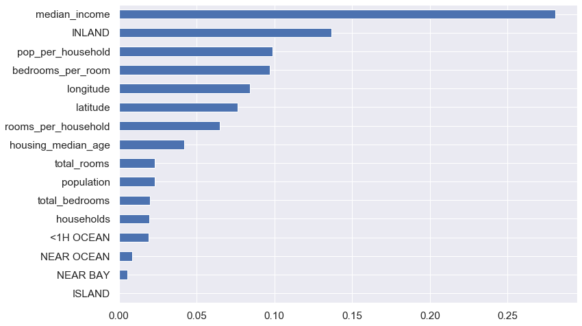

We could drop some features like Island, Near Bay, Near Ocean, <1H Ocean, households, and bedrooms and rerun our model for best result.

metrics.explained_variance_score(y_test, pred2)

0.8252854674155055

Our Random Forest model explain 82.5% of the values.

Next, I will use a Linear Regression model in the future to compare results.